ICP-OES vs ICP-MS: Ultimate Guide to Choosing the Right Analyzer

Fundamental Differences Between ICP‑OES and ICP‑MS: Core Principles Explained

What sets inductively coupled plasma optical emission spectrometry (ICP‑OES) apart from inductively coupled plasma mass spectrometry (ICP‑MS) is the way each instrument turns the plasma’s energy into a measurable signal. In ICP‑OES the plasma excites atoms and ions, causing them to emit light at characteristic wavelengths. A spectrometer isolates those wavelengths and quantifies the intensity, which is proportional to the element concentration. ICP‑MS, by contrast, ionizes the sample in the same plasma but then extracts the ions directly into a mass analyzer—most often a quadrupole or time‑of‑flight (TOF) system. The mass analyzer separates ions based on their mass‑to‑charge ratio (m/z) and counts them with a detector, providing a numerical count that translates into concentration.

Concept → Example → Application

Concept: Light emission vs. mass detection.
Example: When a sodium solution is introduced, ICP‑OES measures the bright yellow line at 589 nm, while ICP‑MS counts ^23Na⁺ ions.
Application: Environmental labs often choose ICP‑OES for routine monitoring of major metals because the emission lines are strong and easy to calibrate. ICP‑MS is preferred for trace‑level contaminants such as lead or arsenic, where counting individual ions down to parts‑per‑trillion is essential.

The physics behind the two techniques further explains their performance gap. Optical emission relies on the plasma’s temperature (typically 8,000–10,000 °C) to populate excited states. The intensity of each line follows the Boltzmann distribution, meaning that elements with low excitation energies produce brighter signals. However, spectral interferences—overlapping lines from different elements—can limit selectivity. Mass spectrometry sidesteps most of these overlaps because each ion is identified by its unique m/z. Yet ICP‑MS must contend with isobaric interferences, where different isotopes share the same nominal mass. Modern collision‑cell technology, often using helium or hydrogen gases, reduces these interferences by kinetic energy discrimination, but the process adds complexity to the instrument.

A practical distinction lies in detection limits. ICP‑OES typically reaches low‑parts‑per‑million (ppm) or, for the strongest lines, low‑parts‑per‑billion (ppb) levels. ICP‑MS routinely pushes into the sub‑ppb regime and can achieve parts‑per‑trillion (ppt) detection for many elements. This sensitivity advantage makes ICP‑MS the go‑to method for compliance testing where regulatory limits are very tight, such as mercury in drinking water.

Another key difference is the type of data each technique provides. ICP‑OES delivers a spectrum that can be visually inspected for unexpected peaks, which aids in troubleshooting and method development. ICP‑MS outputs a mass list that is straightforward to interpret numerically but offers less immediate visual confirmation. For laboratories that value rapid multi‑element screening, ICP‑OES often provides faster run times per sample because the spectrometer can monitor several wavelengths simultaneously without needing to scan a wide mass range.

Historical context → Current state → Future implications When ICP‑OES first entered commercial labs in the 1970s, its simplicity and robustness made it the workhorse for metal analysis. ICP‑MS arrived later, benefiting from advances in vacuum technology and detector electronics that made high‑resolution mass analysis affordable. Today, hybrid instruments combine both emission and mass detection in a single platform, giving users the flexibility to switch modes depending on the analytical need. Looking ahead, improvements in high‑resolution optics and miniaturized plasma sources may narrow the gap in detection limits, while ongoing developments in collision‑cell design promise even cleaner mass spectra for ICP‑MS.

In summary, the fundamental divide rests on how each technique captures the plasma’s output—light versus ions. This core principle influences everything from sensitivity and selectivity to ease of use and cost. Understanding these distinctions helps analysts choose the right tool for their specific analytical challenges, whether they are measuring bulk metals in alloys or detecting trace contaminants in complex environmental samples.

Transition: With the core principles clarified, the next section will explore how each analyzer physically generates data, detailing the key components and operational mechanics that turn plasma energy into measurable results.

How Each Analyzer Generates Data: Key Components and Operational Mechanics

Both ICP‑OES and ICP‑MS share a plasma source, yet the paths the sample takes from introduction to data output diverge dramatically. Understanding these pathways helps users appreciate why one instrument may excel in a particular workflow while the other shines elsewhere.

Core pathway in ICP‑OES

Sample introduction – A nebulizer creates a fine aerosol from the liquid sample, which is carried by argon gas into the plasma torch.
Excitation in the plasma – The high‑temperature (≈10 000 °C) plasma strips electrons from atoms, promoting them to excited states.
Emission of photons – As excited atoms relax, they emit photons at wavelengths that are characteristic of each element.
Wavelength‑dispersive detection – A diffraction grating (or in some designs, a prism) separates the light into its component wavelengths. Photomultiplier tubes or solid‑state detectors capture the intensity of each selected line.
Signal conversion – The detector current is amplified, digitized, and sent to the instrument’s software, where calibration curves translate intensity into concentration.

Because ICP‑OES measures light directly, each element’s signal is tied to a specific wavelength. This straightforward chain makes the technique well suited for routine multi‑element surveys where speed and simplicity are paramount.

Core pathway in ICP‑MS

Sample introduction – Like OES, the sample is nebulized and transported into the plasma, but the subsequent handling differs.
Ion formation – Within the plasma, atoms are ionized to form singly charged positive ions (A⁺). In some instruments a collision/reaction cell may be added to reduce polyatomic interferences.
Mass analysis – The ion beam exits the plasma and is steered into a mass spectrometer. Quadrupole, time‑of‑flight (TOF), or magnetic sector analyzers separate ions based on their mass‑to‑charge ratio (m/z).
Detection – After separation, ions strike a detector—commonly an electron multiplier or an inductively coupled detector—producing a current proportional to ion abundance.
Data processing – The software applies isotope‑specific calibration, background subtraction, and, when needed, mathematical corrections for interferences, delivering concentration values with parts‑per‑trillion precision.

Since ICP‑MS counts ions rather than photons, it can discriminate between isotopes of the same element, offering unrivaled sensitivity for trace analysis.

Shared components that shape data quality

Nebulizer and spray chamber – Both instruments rely on consistent aerosol generation. Poor nebulizer performance introduces variability that propagates through the entire measurement chain.
Torch and plasma power – The stability of the plasma temperature determines excitation efficiency in OES and ionization efficiency in MS. Modern controllers maintain plasma power within ±1 % to reduce drift.
Autosampler – Automated sample handling minimizes human error and ensures that each injection experiences the same residence time, a crucial factor for reproducibility.

Operational nuances that influence the final readout

Wavelength interferences vs. isobaric interferences – In OES, overlapping emission lines can mask a target element; careful selection of alternative lines or background correction helps. In MS, isobaric ions (different elements with the same nominal mass) are addressed through collision/reaction gas chemistry or high‑resolution sector analyzers.
Dynamic range handling – OES typically offers a linear dynamic range of three orders of magnitude per element, while MS can extend to six or more, but both require dilution or a detector‑gain adjustment when concentrations exceed the linear region.
Calibration strategy – Multi‑element standards are common for OES, whereas MS often uses element‑specific internal standards (e.g., indium for trace metals) to correct for matrix effects and instrument drift.

“The choice between measuring photons or counting ions determines not only sensitivity but also the complexity of data correction,” notes a senior analytical chemist familiar with both platforms.

Practical tip for users transitioning between the two

When moving from an OES workflow to an MS workflow, begin by validating the nebulizer‑torch‑autosampler train on a familiar matrix. Then, introduce the mass spectrometer stepwise: first verify that the ion lens voltages transmit the expected ion current, next confirm isotope ratios using a certified reference material, and finally implement interference correction protocols. This staged approach preserves data integrity while capitalizing on the MS’s superior detection limits.

With these mechanisms in mind, the next section will explore how the distinct data generation pathways translate into measurable performance differences such as sensitivity, detection limits, and analysis speed.

Performance Metrics Compared: Sensitivity, Detection Limits, and Speed

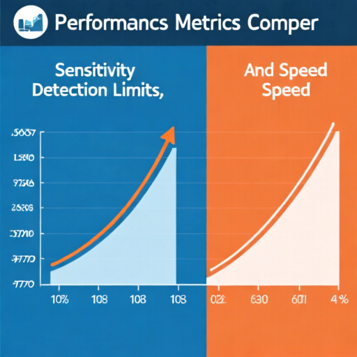
When thelaboratory team moves from theory to practice, three performance characteristics dominate the decision‑making process: sensitivity, detection limits, and analysis speed. Each metric tells a different story about how ICP‑OES and ICP‑MS will behave under real‑world workloads, and understanding their interplay helps prevent costly mismatches between instrument capability and sample demand.

Sensitivity – how much signal a technique can generate from a given amount of analyte

ICP‑OES measures the intensity of light emitted by excited atoms, while ICP‑MS counts individual ions produced in a plasma. Because ion counting is inherently more direct, ICP‑MS typically delivers higher raw sensitivity. In practice, this means that a trace element present at parts‑per‑billion (ppb) levels will generate a clear signal on an ICP‑MS detector, whereas ICP‑OES may require a higher concentration—often a few ppb—to produce a comparable peak.

A practical illustration helps to put this into perspective. Imagine a water‑quality lab that needs to track lead at 5 µg L⁻¹. With an ICP‑MS, the instrument can often detect that concentration in a single scan, producing a crisp peak that is easy to quantify. Using ICP‑OES, the same lab might need to increase the sample introduction flow or perform multiple replicate scans to achieve a reliable measurement. The trade‑off is clear: ICP‑MS offers stronger signal per atom, but ICP‑OES can still meet many routine monitoring requirements if the analyte concentration sits comfortably above its sensitivity threshold.

Detection Limits – the smallest amount that can be reliably distinguished from background noise

Detection limit (DL) is closely tied to sensitivity, but it also reflects the background noise level and instrument stability. ICP‑MS routinely reaches sub‑ppb or even parts‑per‑trillion (ppt) DLs for a wide range of elements, thanks to the low background of mass‑spectrometric detection. For elements that are notoriously challenging—such as arsenic or mercury—ICP‑MS can isolate the isotope of interest and suppress interferences, pushing DLs to levels that meet the strictest regulatory guidelines.

ICP‑OES, by contrast, generally delivers DLs in the low‑ppb range. The optical emission background, especially from matrix gases, can raise the noise floor. Nevertheless, modern ICP‑OES instruments equipped with high‑resolution spectrometers and optimized nebulizers have narrowed the gap. In many environmental applications, a DL of 1–2 ppb is sufficient, making ICP‑OES a cost‑effective alternative when ultra‑trace detection is not a requirement.

Speed – how quickly a sample can be processed from introduction to result

Speed is often the decisive factor for high‑throughput labs. ICP‑MS excels in rapid data acquisition because the detector can record multiple isotopes simultaneously, and modern software can process the ion counts in near‑real time. A typical ICP‑MS run, including plasma stabilization and background correction, can finish in 1–2 minutes per sample.

ICP‑OES, however, may require slightly longer dwell times to achieve acceptable signal‑to‑noise ratios, especially for low‑concentration elements. A full elemental scan on a conventional ICP‑OES system often takes 3–5 minutes, though multi‑element methods can reduce this by focusing on a subset of wavelengths. The difference becomes more pronounced when considering sample preparation steps; both techniques share similar digestion and dilution protocols, so the instrument’s intrinsic scan time is the primary speed differentiator.

Balancing the three metrics for real‑world decisions

When ultra‑low detection limits are non‑negotiable (e.g., trace metal monitoring in drinking water), prioritize ICP‑MS for its superior sensitivity and DLs.
When the target concentration comfortably exceeds the ppb range and the lab processes dozens of samples per hour, ICP‑OES may provide adequate performance while delivering a simpler workflow.
When both speed and multi‑element coverage are needed, consider the instrument’s scan configuration. ICP‑MS can monitor dozens of isotopes in a single run, but ICP‑OES can still achieve respectable throughput with carefully selected emission lines.

A common approach in many analytical labs is to run a “screening” method on ICP‑OES for routine elements and reserve ICP‑MS for confirmatory or regulatory‑driven analyses that demand the lowest possible detection limits.

Understanding the nuanced differences in sensitivity, detection limits, and speed allows practitioners to match each technology to the specific analytical challenge at hand. The next section will explore how these performance traits translate into concrete application choices, from metal alloys to complex geological matrices.

Choosing the Right Technique for Specific Applications: Metals, Trace Elements, and Complex Matrices

Choosingthe Right Technique for Specific Applications: Metals, Trace Elements, and Complex Matrices

When it comes to selecting an analytical method, the chemistry of the sample often dictates the choice. Metals present in high concentrations, trace elements that exist near parts‑per‑billion levels, and samples that contain interfering substances each pose distinct challenges. Understanding how inductively coupled plasma optical emission spectrometry (ICP‑OES) and inductively coupled plasma mass spectrometry (ICP‑MS) respond to these challenges helps laboratories make informed decisions.

Metals in pure or relatively simple matrices – For bulk metal analysis, such as alloy certification or steel grade verification, ICP‑OES typically offers the most straightforward solution. The technique directly measures the characteristic light emitted by each element, providing rapid read‑outs for dozens of metals in a single run. Because the emission lines are strong and the background is low in clean metal solutions, detection limits are often sufficient for quality‑control specifications that sit well above the parts‑per‑million range. Moreover, the robust sample introduction system tolerates the high dissolved solids commonly found in acid‑digested metal streams, reducing the risk of clogging or contamination.

Trace elements in environmental and biological samples – When the target analytes hover near the parts‑per‑billion concentration, ICP‑MS becomes the method of choice. Its ability to separate ions by mass-to-charge ratio delivers detection limits that are an order of magnitude lower than most ICP‑OES configurations. This sensitivity is crucial for monitoring pollutants like arsenic in drinking water, cadmium in food crops, or mercury in fish tissue. In practice, laboratories often employ collision‑reaction cell technology within ICP‑MS to mitigate polyatomic interferences that would otherwise inflate background signals. The result is a cleaner spectrum and more reliable quantification of ultra‑trace species.

Complex matrices rich in organics, salts, or surfactants – Samples such as seawater, waste‑water effluent, or pharmaceutical formulations contain constituents that can suppress the plasma or introduce spectral interferences. ICP‑OES can still be viable if robust matrix‑matching or internal‑standard calibration is applied, but the analyst must accept a higher limit of detection and potentially longer run times due to the need for dilution or chemical separation. ICP‑MS, on the other hand, often handles complex matrices more gracefully. The mass‑based detection is less susceptible to spectral overlap, and modern instruments incorporate high‑resolution or dynamic reaction cell modes that actively remove interfering ions. However, matrix load can still affect ion transmission efficiency, so careful sample preparation—such as microwave digestion followed by filtration—is recommended to preserve instrument performance.

Practical considerations for method selection

Speed vs. sensitivity – If throughput is the primary driver—like routine alloy inspections—ICP‑OES can process dozens of samples per hour with minimal downtime. When the laboratory’s priority is detecting minute contaminants, the slower acquisition time of ICP‑MS is justified by its superior sensitivity.
Elemental coverage – ICP‑OES readily quantifies most transition metals but may struggle with non‑metals that have weak emission lines (e.g., selenium). ICP‑MS excels across the periodic table, including light elements such as lithium and boron, provided the instrument’s detector is tuned appropriately.
Cost of analysis – Sample preparation steps dominate the overall expense. ICP‑OES often requires fewer consumables because it tolerates higher acid concentrations; ICP‑MS may need cleaner reagents and additional gas supplies for collision‑cell operation. Budget constraints can therefore tip the balance toward OES for high‑volume, low‑complexity work.
Regulatory compliance – Certain certification programs (e.g., ISO 17025 for trace element analysis) specifically mandate the use of ICP‑MS to meet stringent detection limit requirements. Laboratories aiming for accreditation should align their method choice with those standards.

Illustrative workflow

Assess the analyte concentration range – Determine whether the expected levels fall within ppm (parts per million) or lower.
Evaluate matrix complexity – Identify high‑salt, high‑organic, or surfactant content that could affect plasma stability.
Match the technique to the need – Choose ICP‑OES for high‑concentration metals in simple matrices; select ICP‑MS for trace elements or challenging matrices.
Implement appropriate preparation – Apply dilution, digestion, or separation steps that complement the chosen analyzer’s strengths.

By aligning the analytical challenge with the inherent capabilities of each plasma‑based instrument, laboratories can achieve reliable results while optimizing resource use. The next logical step is to examine the financial and maintenance implications of each technology, ensuring that the chosen solution fits both the scientific and budgetary goals of the lab.

Cost, Maintenance, and Practical Considerations: Budgeting Your Lab Investment

When the technical merits of ICP‑OES and ICP‑MS have been weighed, the next question many laboratories face is whether the purchase fits within their financial roadmap. While performance often drives the initial choice, total cost of ownership (TCO) can shift the balance dramatically. Understanding the components that contribute to TCO helps decision‑makers allocate resources wisely and avoid unexpected expenses down the road.

Initial acquisition cost is the most visible line item. ICP‑OES instruments typically range from mid‑to‑high‑three‑figure thousands of dollars, making them accessible for most mid‑size labs. ICP‑MS systems, by contrast, start in the high‑four‑figure range and can exceed six figures when equipped with collision/reaction cells or high‑resolution optics. For a laboratory with a tight capital budget, the lower entry price of OES may be tempting, but it is essential to consider whether the analytical limits it offers align with the intended workload.

Beyond the purchase price, operational expenses quickly become a substantial part of the budget. ICP‑MS consumes more argon gas per hour because the plasma operates at higher power and often runs a secondary gas (e.g., helium or nitrogen) for interference reduction. In practice, argon usage can add several thousand dollars per year to the operating budget. ICP‑OES also requires argon, but the flow rates are lower, translating into modest gas costs. Consumables such as nebulizers, cones, and torch components wear out at different rates; ICP‑MS typically replaces these parts more frequently due to the harsher plasma environment.

Maintenance contracts provide another layer of cost transparency. Vendors commonly offer tiered service agreements that cover routine calibration, preventive maintenance visits, and emergency repairs. A basic contract for an ICP‑OES system may run a few thousand dollars annually, whereas a comparable plan for ICP‑MS often approaches double that amount. Laboratories that lack in‑house expertise in mass spectrometry may find the higher service fee a worthwhile trade‑off for reduced downtime.

Space and infrastructure requirements also influence budgeting decisions. ICP‑MS demands a stable power supply, often with dedicated UPS (uninterruptible power supply) units, and enhanced ventilation to handle the higher heat load. Installing these utilities can add \(5,000–\)10,000 to the project cost, especially in older facilities. ICP‑OES systems have a smaller footprint and lower power draw, making them easier to fit into existing bench space without substantial retrofitting.

Training and personnel costs should not be overlooked. Operating an ICP‑MS safely and accurately typically requires a higher level of expertise, especially when dealing with complex collision‑cell methods or high‑resolution modes. A lab may need to invest in specialized training courses, which can range from \(1,000 to \)3,000 per analyst. ICP‑OES, with its more straightforward calibration routines, usually shortens the learning curve, allowing new users to become productive faster.

To help prioritize spending, consider the following checklist:

Define analytical needs: Identify the detection limits, element range, and matrix complexity required for routine work.
Map out consumable usage: Estimate annual argon consumption and replaceable part lifetimes for each instrument type.
Assess available space and utilities: Verify power capacity, ventilation, and floor load before finalizing a purchase.
Plan for service and training: Include contract fees and training courses in the first‑year budget to avoid hidden costs.
Calculate total cost over 5‑year horizon: Add acquisition, consumables, service, utilities, and personnel expenses to compare the true expense of each option.

By approaching the purchase as a long‑term investment rather than a one‑time expense, laboratories can align their analytical capabilities with realistic financial constraints. The next section will build on these considerations, presenting a decision‑making framework that integrates cost, performance, and workflow factors to guide a balanced selection process.

Optimizing Your Choice: Decision‑Making Framework and Best‑Practice Tips

Transitioning from the cost and maintenance discussion, it is now time to layer those financial realities onto the scientific and operational factors that truly drive a successful purchase. A structured decision‑making framework helps laboratories balance budget constraints with performance requirements, while best‑practice tips keep the process efficient and future‑proof.

A step‑by‑step framework

Define the analytical objective – List the elements, concentration ranges, and matrix types that will be measured most frequently. Clarify whether ultra‑trace detection, rapid screening, or simultaneous multi‑element analysis is the primary goal.
Score critical performance criteria – Assign a weight (e.g., 1‑5) to sensitivity, speed, dynamic range, and interference resistance based on the objectives. For a laboratory focused on trace heavy‑metal monitoring in water, sensitivity and low detection limits receive the highest weight; for alloy certification, speed and dynamic range may dominate.
Map requirements to instrument capabilities – Match the weighted scores against the known strengths of ICP‑OES (robustness, lower upfront cost, excellent multi‑element speed) and ICP‑MS (superior detection limits, isotope discrimination, higher susceptibility to matrix effects). This side‑by‑side comparison often reveals a clear front‑runner.
Factor in lifecycle costs – Incorporate consumables, gas usage, calibration standards, and routine service contracts. Even when the purchase price favors ICP‑OES, the higher per‑run consumable cost of ICP‑MS can become significant in high‑throughput labs.
Risk assessment – Identify potential future needs such as new regulatory limits or emerging contaminants. An instrument with modular upgrade paths (e.g., collision/reaction cell for ICP‑MS) may mitigate future risk.

Pro tip: Document each scoring decision in a shared spreadsheet; this not only adds transparency but also creates a reference point if staff turnover occurs.

Best‑practice tips for a smooth selection process

Engage end‑users early. Analysts who will run the instrument daily know practical pain points—such as sample preparation bottlenecks or software ergonomics—that senior management may overlook. Conduct short interviews or a quick survey before finalizing criteria.
Visit reference labs. Seeing an ICP‑OES or ICP‑MS in action provides insight into real‑world uptime, maintenance workflows, and staff training demands. Ask about unexpected downtime causes; many labs cite routine nebulizer clogging or detector drift that were not highlighted in vendor specs.
Pilot with a rental or short‑term lease. A 2‑ to 3‑month trial can validate detection limits on actual samples and reveal hidden consumable consumption rates. Leverage the vendor’s technical support during this phase to gauge responsiveness—a critical factor when troubleshooting complex matrices.
Standardize sample preparation. Even the most sensitive ICP‑MS cannot compensate for poor digestion or filtration practices. Establish a SOP (standard operating procedure) that aligns with the chosen instrument’s tolerances; this improves reproducibility and reduces instrument wear.
Plan for training and knowledge transfer. Allocate budget not only for the instrument but also for certified training courses. Many manufacturers offer onsite workshops that cover calibration, troubleshooting, and software customization, which accelerates competence and reduces early‑stage errors.
Build a maintenance schedule that mirrors usage patterns. For high‑throughput environments, schedule preventive service after a set number of runs rather than calendar time alone. This proactive approach limits unexpected breakdowns that could disrupt critical projects.
Leverage data management tools. Modern ICP systems integrate with LIMS (Laboratory Information Management Systems). Ensure the chosen analyzer supports open data formats (e.g., CSV, XML) to simplify downstream reporting and regulatory compliance.

Putting it all together

When the weighted scoring matrix points to one technology, run a quick “what‑if” scenario: adjust the weight of a single criterion (such as future trace‑element needs) and observe how the recommendation shifts. This sensitivity analysis reveals how robust the decision is and highlights any hidden dependencies.

Finally, record the rationale behind the final choice in a concise decision log. Include the objective list, weighting scheme, cost breakdown, and any risks identified. This log becomes a living document that can be revisited when the laboratory expands, when new analytes emerge, or when budget cycles demand re‑evaluation.

By following this structured framework and applying the practical tips above, laboratories can move beyond intuition and make a clear, defensible choice between ICP‑OES and ICP‑MS—maximizing scientific output while safeguarding the investment over the instrument’s entire lifespan.

My Chemistry